When I study motion in physics, I find that kinematic equations provide one of the clearest ways to connect time, displacement, velocity, and acceleration. These equations allow us to describe how an object moves without first needing to analyze the forces responsible for that motion. In my view, that separation makes kinematics one of the most useful starting points for understanding mechanics.
Kinematic equations are especially important when acceleration remains constant. Under that condition, a small group of equations can describe a surprisingly wide range of situations, including accelerating cars, falling objects, objects sliding along surfaces, and many introductory projectile-motion problems. OpenStax identifies these equations as relationships among time, displacement, velocity, and acceleration under constant acceleration.
The most important lesson I want to emphasize is that memorizing equations alone is not enough. We need to understand what every variable means, recognize which quantities are known, identify the unknown quantity, establish a consistent direction, and then choose an equation that actually fits the information available.
For example, if I know an object’s initial velocity, acceleration, and elapsed time, I can determine its final velocity without knowing its displacement. If I instead know its initial velocity, acceleration, and displacement but not its time, another equation becomes much more useful. The equations are connected, but each one has a particular practical advantage.
Key Takeaways About Kinematic Equations
From my analysis, the most useful principles can be summarized in a few points.
- Kinematic equations describe motion rather than the forces causing that motion.
- The standard equations apply directly to one-dimensional motion with constant acceleration.
- The main variables are initial velocity, final velocity, acceleration, displacement, and time.
- Direction matters because velocity, acceleration, and displacement can be positive or negative.
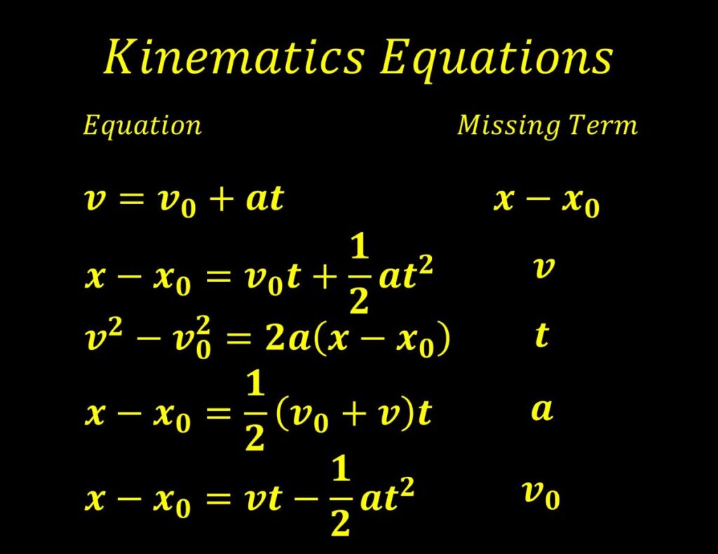
- The equation (v=v_0+at) is particularly useful when time is known and final velocity is required.
- The equation (x=x_0+v_0t+\frac{1}{2}at^2) is useful when displacement is connected to time and acceleration.
- The equation (v^2=v_0^2+2a(x-x_0)) is especially valuable when time is not known.
- A consistent system of units is essential.
- Constant acceleration is an assumption, not a universal property of every moving object.
- Graphs provide another way to understand and check the equations.
We can reasonably conclude that successful kinematics problem solving depends as much on interpreting a situation correctly as it does on performing algebra correctly.
What Kinematic Equations Mean in Physics
Kinematics is the branch of mechanics concerned with describing motion. It focuses on quantities such as position, displacement, velocity, acceleration, and time. It does not, by itself, explain why an object accelerates. Questions about forces belong to dynamics.
In my view, this distinction is important because beginners sometimes mix the two subjects. If a car accelerates from a traffic light, kinematics can tell us how its velocity and position change if the acceleration is known. Newton’s laws can then help explain what forces are responsible for that acceleration.
The basic variables used in one-dimensional kinematics include:
- (x): position
- (x_0): initial position
- (\Delta x): displacement
- (v_0): initial velocity
- (v): final velocity
- (a): acceleration
- (t): elapsed time
Displacement is the change in position:
[
\Delta x=x-x_0
]
Average velocity is displacement divided by elapsed time:
[
v_{\text{avg}}=\frac{\Delta x}{\Delta t}
]
Average acceleration is the change in velocity divided by the elapsed time:
[
a_{\text{avg}}=\frac{\Delta v}{\Delta t}
]
For constant acceleration, average and instantaneous acceleration have the same value. OpenStax explains that taking the initial time as zero simplifies the notation by allowing initial values to carry a subscript of zero while final values can be written without one.
Displacement Is Not the Same as Distance
I believe one of the most important distinctions to understand early is the difference between distance and displacement.
Distance describes the total path length traveled. Displacement describes the change from an initial position to a final position and includes direction.
Suppose, as a hypothetical example, a student walks 50 meters east and then 20 meters west. The total distance traveled is 70 meters. The displacement, however, is 30 meters east.
This distinction becomes important because kinematic equations generally work with displacement or position rather than simply total path distance.
Velocity Is Not the Same as Speed
Speed tells us how quickly an object moves, while velocity includes direction.
A car traveling at 20 m/s east has a velocity of (+20) m/s if east has been chosen as positive. A car traveling at 20 m/s west could have a velocity of (-20) m/s under the same coordinate convention.
From my perspective, signs are not merely mathematical decorations. They communicate physical direction.
The Five Core Kinematic Equations
The familiar set of kinematic equations describes one-dimensional motion under constant acceleration. OpenStax presents the standard relationships as equations connecting position, average velocity, velocity, acceleration, and time.
Equation 1: Average Velocity
The first relationship is:
[
x=x_0+v_{\text{avg}}t
]
For constant acceleration, average velocity can be expressed as:
[
v_{\text{avg}}=\frac{v_0+v}{2}
]
Therefore, displacement can also be written as:
[
x-x_0=\frac{v_0+v}{2}t
]
This equation is useful when the initial and final velocities are known.
For a hypothetical example, suppose an object starts at 4 m/s and reaches 10 m/s over 3 seconds while maintaining constant acceleration. Its average velocity is:
[
v_{\text{avg}}=\frac{4+10}{2}=7\text{ m/s}
]
The displacement is therefore:
[
\Delta x=7(3)=21\text{ m}
]
Equation 2: Velocity and Time
The second major equation is:
[
v=v_0+at
]
This equation tells us how velocity changes when acceleration remains constant.
If an object begins at 5 m/s and accelerates at 2 m/s² for 4 seconds:
[
v=5+(2)(4)
]
[
v=13\text{ m/s}
]
I find this equation especially straightforward because it directly expresses the effect of acceleration over time.
Equation 3: Displacement, Initial Velocity, Acceleration, and Time
The displacement equation is:
[
x=x_0+v_0t+\frac{1}{2}at^2
]
If we focus only on displacement:
[
\Delta x=v_0t+\frac{1}{2}at^2
]
when the initial position is taken as zero.
This equation combines two effects. The term (v_0t) represents displacement that would occur from the initial velocity alone, while the (\frac{1}{2}at^2) term accounts for the additional displacement associated with constant acceleration.
Equation 4: Velocity and Displacement Without Time
The fourth commonly used relationship is:
[
v^2=v_0^2+2a(x-x_0)
]
or:
[
v^2=v_0^2+2a\Delta x
]
I consider this one of the most useful equations in practical problem solving because time does not appear in it.
Suppose a vehicle starts at 10 m/s and accelerates at 3 m/s² over a displacement of 20 m. Its final velocity can be calculated directly:
[
v^2=10^2+2(3)(20)
]
[
v^2=100+120=220
]
[
v=\sqrt{220}\approx14.83\text{ m/s}
]
The positive root represents the final speed in this particular setup.
Equation 5: Average Velocity for Constant Acceleration
Another useful expression is:
[
v_{\text{avg}}=\frac{v_0+v}{2}
]
This equation is specifically applicable to constant acceleration. It is often combined with the displacement relationship:
[
\Delta x=v_{\text{avg}}t
]
Substitution gives:
[
\Delta x=\frac{v_0+v}{2}t
]
These equations are not isolated formulas. They form a connected system. OpenStax emphasizes that the equations are not independent and that a problem may require more than one equation when multiple unknowns exist.
Why Constant Acceleration Matters
The phrase “constant acceleration” is the condition I would check before applying the standard kinematic equations.
Constant acceleration means that acceleration does not change with time. OpenStax defines constant acceleration as acceleration that does not change with respect to time.
A hypothetical object that increases its velocity by 3 m/s every second has constant acceleration of 3 m/s². Its velocity might progress like this:
| Time | Velocity |
|---|---|
| 0 s | 0 m/s |
| 1 s | 3 m/s |
| 2 s | 6 m/s |
| 3 s | 9 m/s |
| 4 s | 12 m/s |
The velocity changes by the same amount during each equal time interval.
By contrast, if the velocity increases by 2 m/s during one second, then 5 m/s during the next, and 1 m/s during the following second, the acceleration is not constant.
This does not mean that kinematics becomes impossible when acceleration varies. It means that the simple constant-acceleration equations cannot automatically be applied to the entire motion. The motion may instead need to be analyzed with more general relationships or divided into intervals where a constant-acceleration approximation is reasonable.
OpenStax notes that when acceleration changes significantly, motion can sometimes be considered in separate portions, with each portion having its own constant acceleration.
Understanding the Equations Through Graphs
I believe graphs make kinematic equations much easier to understand because they show the relationships visually.
A position-time graph describes how position changes as time passes. The slope of a position-time graph represents velocity.
A velocity-time graph provides another important relationship. Its slope represents acceleration, while the area under the graph represents displacement for the relevant interval.
A constant-acceleration situation produces a straight-line velocity-time graph because the velocity changes at a constant rate.
The relationship
[
v=v_0+at
]
can therefore be interpreted as the equation of a straight line. Here, (v_0) acts like the intercept and (a) acts like the slope.
For displacement, the equation
[
\Delta x=v_0t+\frac{1}{2}at^2
]
contains a squared time term. This is why position does not generally change linearly with time when acceleration is constant and nonzero.
OpenStax similarly describes the slope of a velocity-time graph as acceleration and connects the equations to graphical representations of motion.
Practical Applications of Kinematic Equations
Kinematic equations appear in many educational and practical contexts. I would not describe them as equations used only for textbook exercises. They provide a mathematical model for many types of approximately constant-acceleration motion.
Accelerating Vehicles
A common example involves a vehicle starting from rest.
Suppose a car starts from rest and accelerates at 2.5 m/s² for 8 seconds.
The initial velocity is:
[
v_0=0
]
The final velocity becomes:
[
v=0+(2.5)(8)=20\text{ m/s}
]
The displacement is:
[
\Delta x=0(8)+\frac{1}{2}(2.5)(8^2)
]
[
\Delta x=80\text{ m}
]
This is a hypothetical calculation, not a claim about a particular vehicle.
Braking Problems
Kinematic equations can also describe slowing motion.
Suppose a vehicle travels at 24 m/s and decelerates at 6 m/s². If we choose the direction of travel as positive, then:
[
v_0=24\text{ m/s}
]
[
v=0
]
[
a=-6\text{ m/s}^2
]
Using:
[
v^2=v_0^2+2a\Delta x
]
we obtain:
[
0^2=24^2+2(-6)\Delta x
]
[
0=576-12\Delta x
]
Therefore:
[
\Delta x=48\text{ m}
]
The result means the object travels 48 meters during the modeled braking interval.
Falling Objects
Vertical motion under gravity is another major application. Near Earth’s surface, when air resistance is neglected, the acceleration due to gravity is commonly approximated as (9.80\text{ m/s}^2). The sign depends on the coordinate system chosen. OpenStax notes that gravity is generally assigned a negative acceleration when upward is selected as the positive direction.
Suppose an object is dropped from rest and falls for 2 seconds. Taking upward as positive:
[
v_0=0
]
[
a=-9.80\text{ m/s}^2
]
The final velocity is:
[
v=0+(-9.80)(2)
]
[
v=-19.6\text{ m/s}
]
The negative sign indicates downward motion according to our chosen coordinate system.
Projectile Motion
Projectile motion requires more care because the motion is usually analyzed separately along horizontal and vertical axes.
For ideal projectile motion near Earth’s surface, horizontal acceleration is often modeled as zero while vertical acceleration is approximately (-9.80\text{ m/s}^2) when upward is positive. OpenStax applies the kinematic equations independently to the horizontal and vertical components of projectile motion.
This is an important example of how a seemingly complicated motion can be broken into simpler one-dimensional problems.
A Quick Comparison of the Main Kinematic Equations
Before solving problems, I recommend comparing the variables present in each equation. This helps prevent the common mistake of selecting an equation simply because it looks familiar.
| Equation | Best Used When | Variables Included |
|---|---|---|
| (v_{\text{avg}}=\frac{v_0+v}{2}) | Initial and final velocities are known | (v_0, v) |
| (\Delta x=v_{\text{avg}}t) | Average velocity and time are known | (\Delta x, v_{\text{avg}}, t) |
| (v=v_0+at) | Time and acceleration are known | (v, v_0, a, t) |
| (\Delta x=v_0t+\frac{1}{2}at^2) | Time, initial velocity, and acceleration are known | (\Delta x,v_0,a,t) |
| (v^2=v_0^2+2a\Delta x) | Time is unknown or unnecessary | (v,v_0,a,\Delta x) |
The most useful takeaway from this table is that I should identify the known and unknown quantities before selecting an equation. The equation containing the fewest unnecessary unknowns is often the easiest starting point.
Step-by-Step Method for Solving Kinematics Problems
I find that a consistent procedure reduces both algebraic errors and conceptual mistakes.
Step 1: Identify the Physical Situation
First, I determine what is actually happening. Is the object speeding up, slowing down, falling, moving upward, or changing direction?
I do not begin by immediately inserting numbers into an equation.
Step 2: Choose a Positive Direction
Next, I establish a coordinate direction.
For horizontal motion, I might choose right as positive. For vertical motion, I might choose upward as positive.
Once I choose that direction, I must use it consistently.
Step 3: List the Known Quantities
I write down:
[
v_0,\quad v,\quad a,\quad t,\quad \Delta x
]
and fill in only the values that are actually given or can be determined.
For example:
[
v_0=12\text{ m/s}
]
[
a=2\text{ m/s}^2
]
[
t=5\text{ s}
]
[
\Delta x=?
]
Step 4: Identify the Unknown
The question may ask for final velocity, displacement, acceleration, or time.
This sounds simple, but I have found that explicitly identifying the unknown often makes equation selection much easier.
Step 5: Select an Appropriate Equation
If I know (v_0), (a), and (t), then:
[
v=v_0+at
]
is an obvious candidate for final velocity.
If I need displacement using those same quantities, then:
[
\Delta x=v_0t+\frac12at^2
]
is appropriate.
If time is not given and I know displacement, then:
[
v^2=v_0^2+2a\Delta x
]
may be the better choice.
Step 6: Substitute With Units
I keep units visible during calculations whenever practical.
For example:
[
v=(8\text{ m/s})+(3\text{ m/s}^2)(4\text{ s})
]
which gives:
[
v=20\text{ m/s}
]
Step 7: Check the Direction and Reasonableness
A final numerical answer is not enough. I ask whether the sign makes physical sense and whether the magnitude is reasonable.
If an object is slowing while moving in the positive direction, a negative acceleration is expected.
Step 8: State the Final Answer Clearly
I include the numerical result and unit, and when direction matters, I state the direction as well.
Worked Example: Finding Final Velocity
Consider a hypothetical cyclist traveling at 6 m/s who accelerates at 1.5 m/s² for 4 seconds.
Known:
[
v_0=6\text{ m/s}
]
[
a=1.5\text{ m/s}^2
]
[
t=4\text{ s}
]
We want (v).
Using:
[
v=v_0+at
]
we obtain:
[
v=6+(1.5)(4)
]
[
v=12\text{ m/s}
]
Therefore, under the stated constant-acceleration assumption, the final velocity is 12 m/s.
The important part is not merely the arithmetic. We can see that the equation was selected because it contains exactly the known quantities needed to determine the unknown velocity.
Worked Example: Finding Displacement
Now consider a hypothetical object starting at 3 m/s and accelerating at 2 m/s² for 5 seconds.
We use:
[
\Delta x=v_0t+\frac12at^2
]
Substituting:
[
\Delta x=(3)(5)+\frac12(2)(5^2)
]
[
\Delta x=15+25
]
The result is 40 meters.
I find this example useful because it shows why the (t^2) term matters. Acceleration contributes increasingly to displacement as time increases.
Worked Example: Solving Without Time
Suppose a hypothetical object has an initial velocity of 4 m/s, accelerates at 2 m/s², and travels 30 meters. We want the final velocity.
Because time is not given, I would choose:
[
v^2=v_0^2+2a\Delta x
]
Substituting:
[
v^2=4^2+2(2)(30)
]
[
v^2=16+120
]
[
v^2=136
]
Therefore:
[
v=\sqrt{136}\approx11.66\text{ m/s}
]
The positive value is appropriate if the object continues moving in the positive direction.
Common Mistakes When Using Kinematic Equations
Using the Equations When Acceleration Is Not Constant
This is perhaps the most important conceptual error.
The standard equations are derived for constant acceleration. OpenStax explicitly states that these kinematic equations apply to constant-acceleration conditions.
If acceleration changes significantly with time, I should not automatically apply the same equation to the entire motion.
Confusing Distance With Displacement
A problem involving a path that changes direction may require careful attention to displacement rather than total distance.
For example, an object traveling 10 meters forward and then 10 meters backward has traveled 20 meters but has zero net displacement.
Losing the Sign of Acceleration
When an object slows while moving in the positive direction, acceleration is negative.
Calling every slowing acceleration “negative” without considering the coordinate system is also incorrect. The sign depends on the chosen direction.
Mixing Units
If velocity is given in kilometers per hour while acceleration is given in meters per second squared, direct substitution creates an inconsistency.
I recommend converting quantities into a consistent unit system before calculating.
Choosing an Equation With Too Many Unknowns
Suppose I know (v_0), (a), and (t), and I want (v). The equation
[
v=v_0+at
]
contains only one unknown.
Choosing another equation that introduces displacement unnecessarily can make the problem harder.
Taking the Wrong Square-Root Sign
When solving:
[
v^2=136
]
mathematically, both positive and negative roots exist.
Physics determines which root is appropriate based on the direction and conditions of the problem.
What the Equations Tell Us About Acceleration
The equation
[
v=v_0+at
]
shows that constant acceleration produces a linear change in velocity with time.
The equation
[
\Delta x=v_0t+\frac12at^2
]
shows that displacement has a quadratic dependence on time when acceleration is nonzero.
The equation
[
v^2=v_0^2+2a\Delta x
]
shows that velocity squared changes linearly with displacement for constant acceleration.
These are not merely algebraic patterns. They describe different mathematical views of the same physical motion.
OpenStax summarizes the purpose of the kinematic equations by explaining that they show how time, displacement, velocity, and acceleration are related.
A particularly useful sourced statement comes from the OpenStax authors because it directly captures the central limitation of the formulas:
“The kinematic equations that we will be using apply to conditions of constant acceleration.”
Paul Peter Urone and Roger Hinrichs, OpenStax
I consider this quotation important because it prevents one of the biggest misunderstandings in introductory physics: treating the equations as universal formulas for every possible type of motion.
How to Decide Which Kinematic Equation to Use
My preferred strategy is to ignore the appearance of the equations at first and focus on the variables.
If time is known and I need final velocity, I look at:
[
v=v_0+at
]
If I need displacement and know time, initial velocity, and acceleration, I use:
[
\Delta x=v_0t+\frac12at^2
]
If time is absent but displacement is known, I consider:
[
v^2=v_0^2+2a\Delta x
]
If initial and final velocity are known and I need displacement, I can use:
[
\Delta x=\frac{v_0+v}{2}t
]
This approach turns equation selection into a variable-matching exercise rather than a memory contest.
Kinematic Equations in Free-Fall Problems
Free-fall problems are often treated as a special application of the same equations.
If upward is positive:
[
a=-g
]
and near Earth’s surface:
[
g\approx9.80\text{ m/s}^2
]
For an object dropped from rest:
[
v_0=0
]
so the displacement equation becomes:
[
\Delta y=-\frac12gt^2
]
The velocity equation becomes:
[
v=-gt
]
These are simplified forms of the general kinematic equations rather than separate laws.
A quotation from the OpenStax treatment of acceleration helps clarify the physical interpretation:
“Gravity is the force that causes nonsupported objects to accelerate downward—or, more precisely, toward the center of Earth.”
Paul Peter Urone and Roger Hinrichs, OpenStax
This matters because the negative sign in a free-fall equation is not saying gravity is inherently “negative.” It reflects the coordinate choice when upward is defined as positive.
Comparing Common Kinematics Situations
The following table helps me distinguish several common applications without treating them as identical physical situations.
| Situation | Typical Acceleration Model | Useful Starting Equation | Main Issue to Watch |
|---|---|---|---|
| Car accelerating in one direction | Approximately constant (a) | (v=v_0+at) | Unit consistency |
| Car braking | Constant negative (a) in an idealized model | (v^2=v_0^2+2a\Delta x) | Correct sign |
| Object dropped vertically | (a=-g) if upward is positive | (v=v_0-gt) | Coordinate direction |
| Object thrown upward | (a=-g) | (v^2=v_0^2-2g\Delta y) | Velocity becomes zero at the top |
| Ideal projectile | (a_x=0,\ a_y=-g) | Apply equations by component | Separate axes |
| Motion with changing acceleration | (a) varies | Standard equations may not apply globally | Need a more general model |
The central takeaway is that the equations remain the same while the physical interpretation of the variables changes according to the situation.
Expert Recommendations for Better Kinematics Problem Solving
From my perspective, the most effective improvement is to slow down the setup rather than rushing through the arithmetic.
First, I recommend drawing a simple diagram. Even a line with an arrow indicating positive direction can prevent sign errors.
Second, I recommend writing every known variable before choosing an equation. This immediately reveals which quantities are missing.
Third, I would keep symbolic expressions until the equation has been selected. Substituting numbers too early can hide conceptual mistakes.
Fourth, I recommend checking dimensions. For example, in:
[
\frac12at^2
]
acceleration has units of m/s² and (t^2) has units of s², leaving meters. That confirms the term can represent displacement.
Fifth, I would use a second method as a check when practical. If I calculate final velocity using (v=v_0+at), I might verify the result through another relationship if enough information is available.
Finally, I believe students should practice explaining why an equation was chosen. Saying “I used this equation because it contains the known initial velocity, acceleration, and time and has final velocity as the only unknown” demonstrates much stronger understanding than simply presenting a numerical answer.
A Reliable Kinematics Checklist
When I approach a new problem, I can use this sequence:
- Read the entire problem before calculating.
- Identify the moving object.
- Determine whether acceleration is constant.
- Select a positive direction.
- Write the known quantities.
- Identify the unknown.
- Convert units if necessary.
- Select an equation containing the required variables.
- Substitute values carefully.
- Solve algebraically.
- Check the sign.
- Check the units.
- Ask whether the result is physically reasonable.
- State the answer clearly.
This process may seem slower at first, but I have found that it generally becomes faster with practice because fewer corrections are required later.
Why Understanding Beats Memorizing Kinematic Equations
I believe memorization has a limited role in physics. It is useful to know the standard equations, but understanding their structure is more powerful.
For example, if I remember that acceleration measures the rate of change of velocity, then:
[
a=\frac{v-v_0}{t}
]
can be rearranged naturally into:
[
v=v_0+at
]
Likewise, understanding average velocity under constant acceleration helps connect velocity and displacement.
The equations are therefore not random formulas that need to be memorized independently. They are connected descriptions of the same physical model.
The OpenStax authors make this broader relationship clear in their treatment of motion:
“The kinematic equations show how time, displacement, velocity, and acceleration are related.”
Paul Peter Urone and Roger Hinrichs, OpenStax
For me, that is the central idea behind learning kinematics effectively. Once the relationships are understood, equation selection becomes much more intuitive.
Conclusion
I believe the most useful way to learn kinematic equations is to treat them as connected descriptions of motion rather than isolated formulas. Their real value becomes clear when we understand the relationships among displacement, velocity, acceleration, and time and recognize that the standard equations require constant acceleration.
In my view, the strongest problem-solving strategy is straightforward: identify the physical situation, choose a coordinate direction, list the known quantities, identify the unknown, select the equation that matches those variables, and then check the result for units, signs, and physical reasonableness. This approach is more reliable than trying to remember which formula “looks right.”
The practical lesson from studying kinematic equations is that mathematics becomes much easier when the physical situation is understood first. We can use the equations for accelerating and braking objects, free fall, and components of projectile motion, provided their assumptions are respected.
As a next step, I recommend practicing several problems that deliberately require different equations. That will help build the ability to recognize which relationship is appropriate rather than simply memorizing a formula.
Frequently Asked Questions
What Are Kinematic Equations?
Kinematic equations are mathematical relationships used to describe motion in terms of quantities such as displacement, velocity, acceleration, and time. The standard equations are most directly applicable when acceleration is constant. They allow us to calculate an unknown motion variable when enough other variables are known. I consider them foundational because they provide a systematic way to analyze one-dimensional motion before introducing more advanced mathematical methods.
What Are the Four Main Kinematic Equations?
The commonly used constant-acceleration relationships include (v=v_0+at), (\Delta x=v_0t+\frac12at^2), (v^2=v_0^2+2a\Delta x), and (\Delta x=\frac{v_0+v}{2}t). A related equation is (v_{\text{avg}}=(v_0+v)/2). Different textbooks may count and organize these relationships slightly differently. The important point is that they form a connected system for constant-acceleration motion.
When Can I Use Kinematic Equations?
You can directly use the standard kinematic equations when the motion being modeled has constant acceleration. Examples include idealized falling objects near Earth’s surface, motion with a specified constant acceleration, and individual segments of a problem where acceleration remains constant. If acceleration changes significantly throughout the interval, the standard equations should not automatically be applied to the entire motion. The problem may require a different mathematical approach.
How Do I Choose the Right Kinematic Equation?
I recommend identifying the known and unknown variables first. If you know initial velocity, acceleration, and time and need final velocity, use (v=v_0+at). If you need displacement and know initial velocity, acceleration, and time, use (\Delta x=v_0t+\frac12at^2).
What Does Negative Acceleration Mean?
Negative acceleration means that the acceleration vector points in the negative direction of the coordinate system. It does not automatically mean an object is slowing down. For example, if an object is moving in the negative direction and has negative acceleration, it may actually be speeding up. I therefore recommend determining the direction of velocity and acceleration before interpreting a negative sign.
Are Kinematic Equations Used for Free Fall?
Yes. Free-fall motion can be modeled with the same kinematic equations when gravitational acceleration is treated as constant. Near Earth’s surface, (g) is commonly approximated as (9.80\text{ m/s}^2). If upward is selected as positive, gravitational acceleration is represented as (-9.80\text{ m/s}^2). The equations then describe the object’s vertical velocity and displacement over time.
Can Kinematic Equations Be Used for Projectile Motion?
Yes, but projectile motion is normally separated into horizontal and vertical components. In an ideal model without air resistance, horizontal acceleration is zero while vertical acceleration is approximately (-9.80\text{ m/s}^2) when upward is positive. The kinematic equations can then be applied independently to each component. This method makes projectile motion easier to analyze because two-dimensional motion is separated into simpler one-dimensional calculations.
Why Is Time Missing From One of the Kinematic Equations?
The equation (v^2=v_0^2+2a\Delta x) is particularly useful because it eliminates time. This makes it valuable when a problem gives initial velocity, acceleration, and displacement but does not provide elapsed time. Rather than introducing an unnecessary variable, I can use the equation directly to connect velocity and displacement.
What Is the Most Common Kinematics Mistake?
One of the most common mistakes is applying a constant-acceleration equation without checking whether acceleration is actually constant. Other frequent problems include confusing distance with displacement, losing negative signs, mixing units, and choosing an equation with unnecessary unknowns. I find that writing down the known variables and selecting a coordinate direction before calculating prevents many of these errors.
Sources and References
- Paul Peter Urone and Roger Hinrichs, Physics, OpenStax, sections covering acceleration and kinematic equations.
- Paul Peter Urone and Roger Hinrichs, University Physics Volume 1, OpenStax, section on motion with constant acceleration.
- OpenStax, College Physics, section on motion equations for constant acceleration in one dimension.
- OpenStax, Physics, section on projectile motion and the application of kinematic equations to motion components.
Disclaimer
This article is intended for educational purposes and provides a general explanation of kinematic equations and constant-acceleration motion. Numerical examples are hypothetical unless explicitly identified as sourced examples. Actual physical systems may involve changing acceleration, air resistance, friction, measurement uncertainty, or other factors that require a more detailed model. Readers should verify assumptions, units, and problem-specific conditions before applying any equation to an engineering, scientific, safety-critical, or real-world situation.